Detect fishing vessel presence within Marine Protected Areas polygons in Mexico

The function spatially joins the Vessels Monitoring System, VMS, points with the Marine Protected Area, MPAs, polygons in Mexico.

Usage

join_mpa_data(x, all_mpas = all_mpas)

Arguments

x

A data.frame with VMS data that must contain columns longitude and latitude

all_mpas

A shape file that contains all MPA polygons in Mexico you can upload this using data("all_mpas")

Value

A data.frame

Details

It adds three columns zone, mpa_decree, state, municipality, region, which are data from the MPAs polygon. zone contains the name of the MPA (in Spanish) and when the vessel is outside an MPA polygon is dubbed as open area, mpa_decree contains the type of MPA (such as National Park, etc.), state contains the Mexican state with jurisdiction on the MPA, municipality contains the Mexican municipality with jurisdiction over the MPA, and region contains the overall location of the MPA (in Spanish)

Examples

# Use sample_dataset
data("sample_dataset")
data("all_mpas")
vms_cleaned <- vms_clean(sample_dataset)
#> Cleaned: 969 empty rows from data! 
vms_mpas <- join_mpa_data(vms_cleaned, all_mpas)
#> although coordinates are longitude/latitude, st_intersects assumes that they
#> are planar
#> although coordinates are longitude/latitude, st_intersects assumes that they
#> are planar


# Plotting data
# Points NOT inside MPA are removed to reduce data size
vms_mpas_sub <- vms_mpas  |>
  dplyr::filter(zone != "open area")

vms_mpas_sf <- sf::st_as_sf(vms_mpas_sub, coords = c("longitude", "latitude"), crs = 4326)

# Loading Mexico shapefile
data("mx_shape")

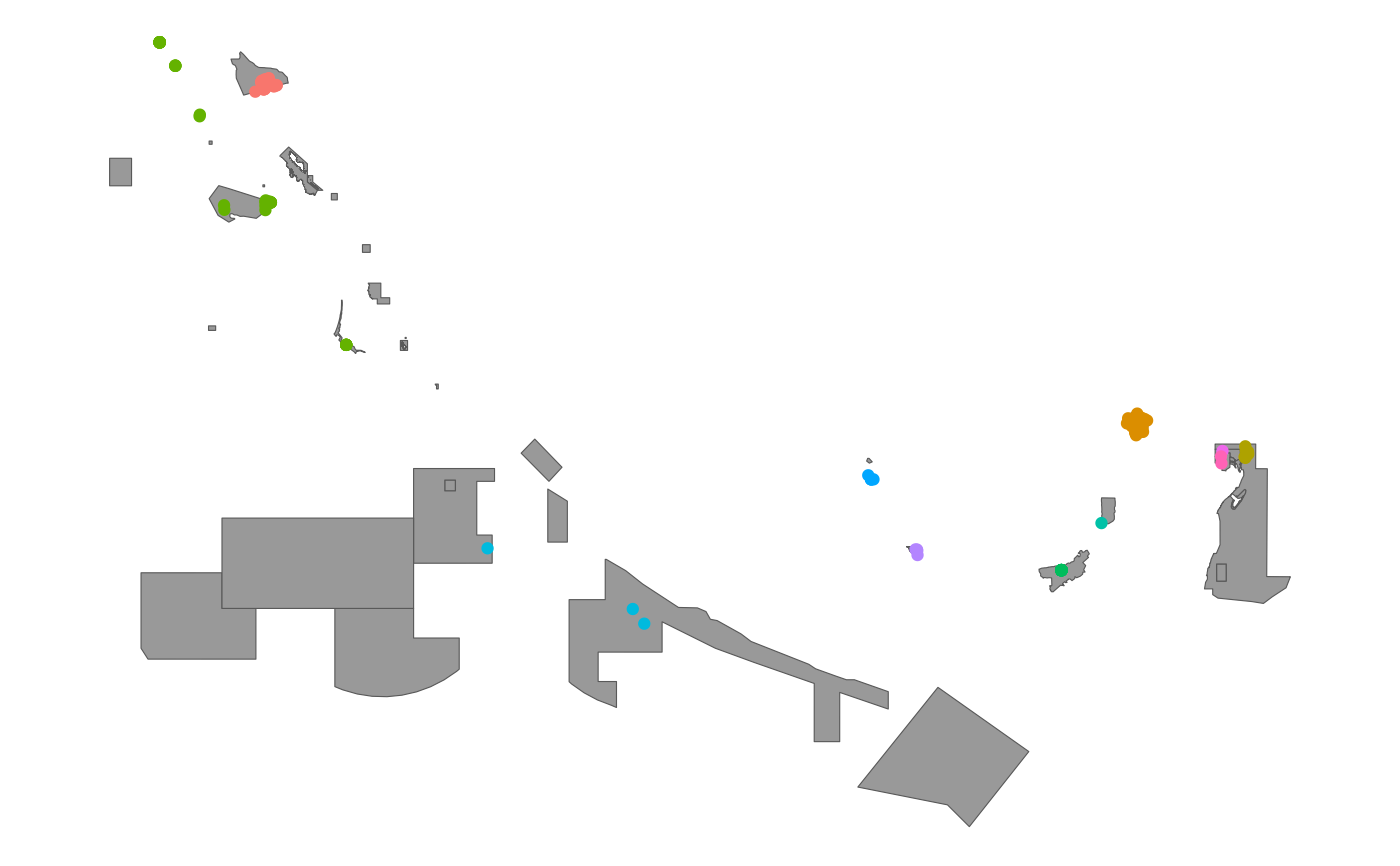
# Map
library(ggplot2)
ggplot(mx_shape, col = "gray90") +
  geom_sf(data = all_mpas, fill = "gray60") +
  geom_sf(data = vms_mpas_sf, aes(col = zone)) +
  theme_void() +
  theme(legend.position = "")